problem13
13. Statics vs Dynamics. 2D. Equilibrium and dynamics of a point mass \(m\) at \(\vec{r}_{C}\). Gravity \(g\) points down in the minus \(\hat{j}\) direction. Points A and B are anchored at \(\vec{r}_A\) and \(\vec{r}_B\). Springs and parallel dashpots connect the mass to A and B. The spring constants are \(k_A\) and \(k_B\). Their rest lengths are \(L_A\) and \(L_B\). Parallel to the springs are dashpots \(c_A\) and \(c_B\). The mass also has a drag force proportional to speed through the air \(c_d\).
The dynamic state of the system is described with \(z = [x, y, \dot{x}, \dot{y}]'\) and the static state by \(z = [x, y, 0, 0]'\).
- Basic Statics. Given parameters and an initial guess, find an equilibrium position of this system. If you have an example you like, post it and people can compare solutions.
- Basic Dynamics. Given parameters and an initial condition, find the motion.
- All equilibria. Given parameters, attempt to find all equilibria. How many are there? By varying parameters, what is the most and least number of equilibrium points there can be?
- Stability of equilibrium. Given an equilibrium point, find it’s stability 2 ways: (a) With a dynamic simulation near the equilibrium; and (b) looking at the eigenvalues of the matrix describing the linearized equations of motion. Compare.
Make appropriate plots, animations and comparisons.
In file ./FindEquilibrium/src/FindEquilibrium.jl:
module FindEquilibrium
import DifferentialEquations
import GLMakie
include("./Physics.jl")
include("Visualization.jl")
struct SpringParameters
k::Float64 # constant
l::Float64 # restlen
r⃗₀::Vector{Float64} # anchor point
c::Float64 # damp: dashpot
end
struct Parameters
m::Float64
g::Float64
c_d::Float64
spring1::SpringParameters
spring2::SpringParameters
end
p = Parameters(
(global m = 0.1),
(global g = 0.1),
(global c_d = 0.5),
(global spring1 = SpringParameters(
(global k1=2.0),
(global l1=2.0),
(global r⃗₁=[1.0, 0.0]),
(global c1=1.0),
)
),
(global spring2 = SpringParameters(
(global k2=1.0),
(global l2=0.5),
(global r⃗₂=[-1.0, -1.0]),
(global c2=1.0),
)
),
)
tspan = (
(global tstart=0.0),
(global tend=200.0)
)
u⃗₀ = [
(global r0=[-1.0;1.0]);
(global v0=[10.0;5.0]);
]
odefunc = Physics.twospringsdragdamped!
odeprob = DifferentialEquations.ODEProblem(
odefunc,
u⃗₀,
tspan,
p,
)
Δt = 0.1
trajectory = GLMakie.Figure()
trajectory_lines = GLMakie.Axis(
trajectory[1,1],
title="Trajectory",
aspect=GLMakie.DataAspect(),
)
i = [1.0;0.0]
j = [0.0;1.0]
N, n = 30, 5
Δr⃗₀s = (global ϵ=0.01)*[cos(θ)*i+sin(θ)*j for θ in range(0.0; step=2π/N, length=n)]
Δd = abs.(r⃗₁ - r⃗₂)
for x in range(min(r⃗₁[1], r⃗₂[1]) - Δd[1], max(r⃗₁[1], r⃗₂[1]) + Δd[2], length=N)
for y in range(min(r⃗₁[2], r⃗₂[2]) - Δd[2], max(r⃗₁[2], r⃗₂[2]) + Δd[2], length=N)
u⃗₀ = [
[x;y];
[0.0;0.0];
]
for Δr⃗₀ in Δr⃗₀s
u⃗₀_modified = u⃗₀ + [Δr⃗₀; Δr⃗₀]
odeprob = DifferentialEquations.ODEProblem(
odefunc,
u⃗₀_modified,
tspan,
p,
)
sol = DifferentialEquations.solve(
odeprob;
# saveat=Δt,
save_everystep=false,
)
# Visualization.plot_trajectory!(trajectory, sol)
# Visualization.plot_start_end!(trajectory, sol)
Visualization.plot_end!(trajectory, sol)
end
end
end
Visualization.plot_points!(trajectory, spring1.r⃗₀, spring2.r⃗₀)
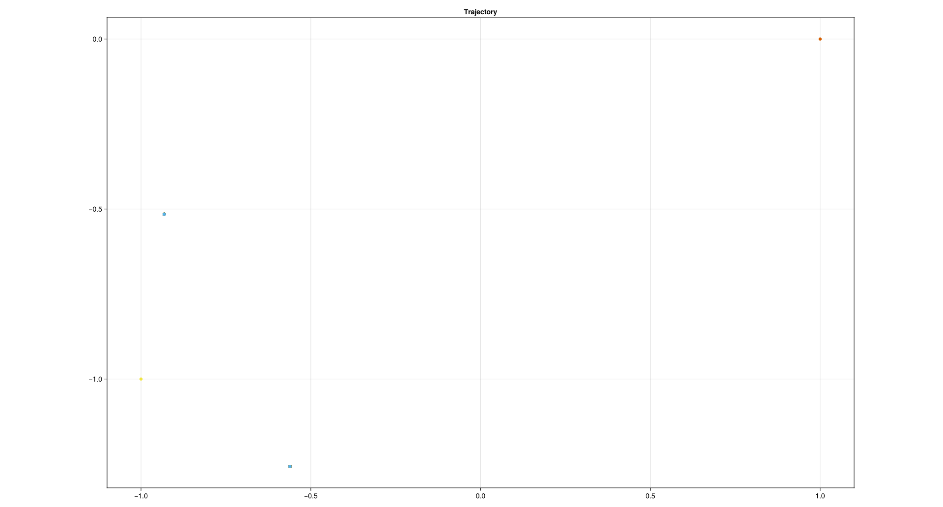
end # module FindEquilibrium(a) Basic Statics. Given parameters and an initial guess, find an equilibrium position of this system. If you have an example you like, post it and people can compare solutions.
Finally, taking the average of the two clusters of end points gives us these equilibrium state.
[[-0.8, -0.49],[-0.6, -1.8]]
Note, The axis aspect are not equal.
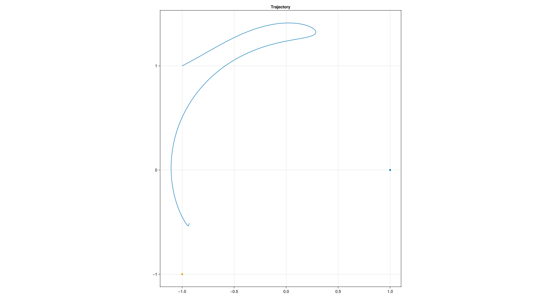
(b) Basic Dynamics. Given parameters and an initial condition, find the motion.
In file ./FindEquilibrium/src/Physics.jl:
module Physics
import LinearAlgebra: norm, normalize, dot
function twospringsdragdamped!(du, u, p, t)
m, g, c_d, spring1, spring2 = p.m, p.g, p.c_d, p.spring1, p.spring2
r⃗ = u[1:2]
v⃗ = u[3:4]
a⃗ = begin
gravity = begin
j = [0.0;1.0]
m*g*(-j)
end
drag = begin
v = norm(v⃗)
v̂ = v⃗/v
(c_d*v)*(-v̂)
end
spring1 = begin
spring = begin
Δr⃗ = r⃗ - spring1.r⃗₀
Δr = norm(Δr⃗)
Δl = Δr - spring1.l
Δr̂ = Δr⃗ / Δr
(spring1.k*Δl)*(-Δr̂)
end
dashpot = begin
r̂ = normalize(r⃗)
(spring1.c*dot(v⃗, r̂))*(-r̂)
end
spring+dashpot
end
spring2 = begin
spring = begin
Δr⃗ = r⃗ - spring2.r⃗₀
Δr = norm(Δr⃗)
Δl = Δr - spring2.l
Δr̂ = Δr⃗ / Δr
(spring2.k*Δl)*(-Δr̂)
end
dashpot = begin
r̂ = normalize(r⃗)
(spring2.c*dot(v⃗, r̂))*(-r̂)
end
spring+dashpot
end
F = +gravity+drag+spring1+spring2
F/m
end
du[1:2] = v⃗
du[3:4] = a⃗
end
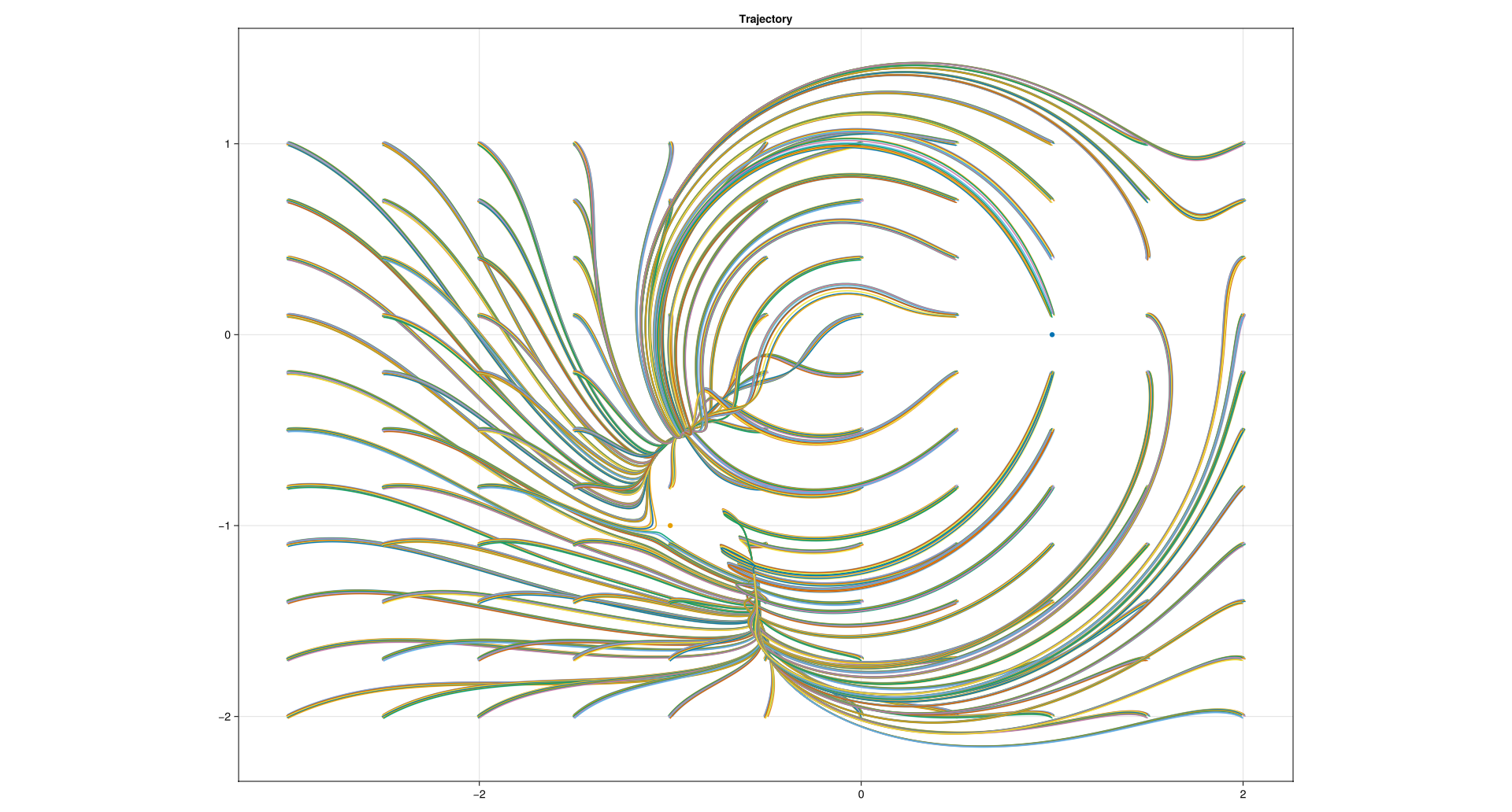
end # module PhysicsAn example trajectory for the taken parameters:
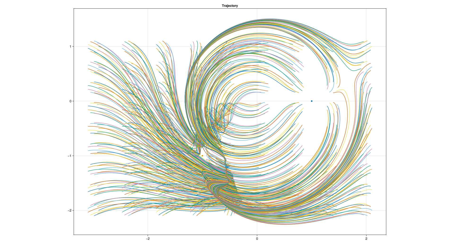
(c) All equilibria. Given parameters, attempt to find all equilibria. How many are there? By varying parameters, what is the most and least number of equilibrium points there can be?
What I did essentially was to take many (about 300) intial position vectors in a grid around the and containing the anchor points. I tried various methods, but essentially all of the methods revolved around playing the simulation and noting the end point. Look at some of the plots below:
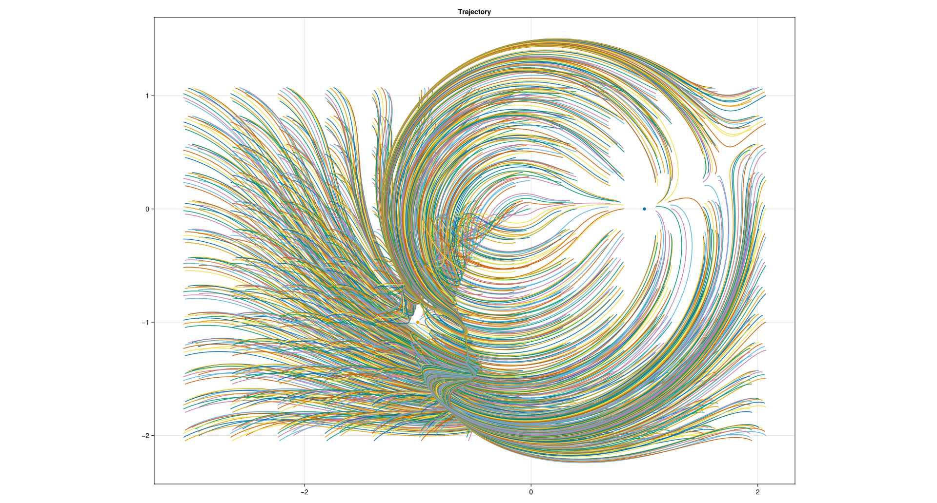
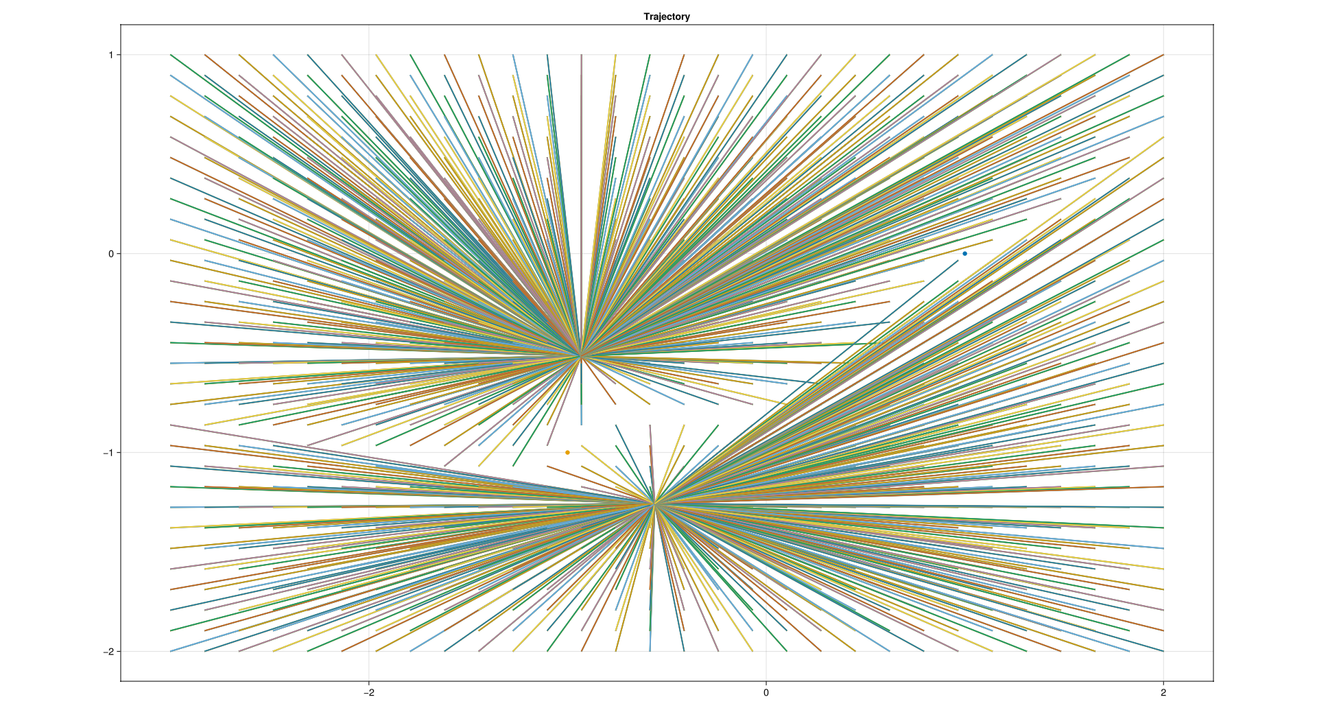
Trying to use a negative air drag:


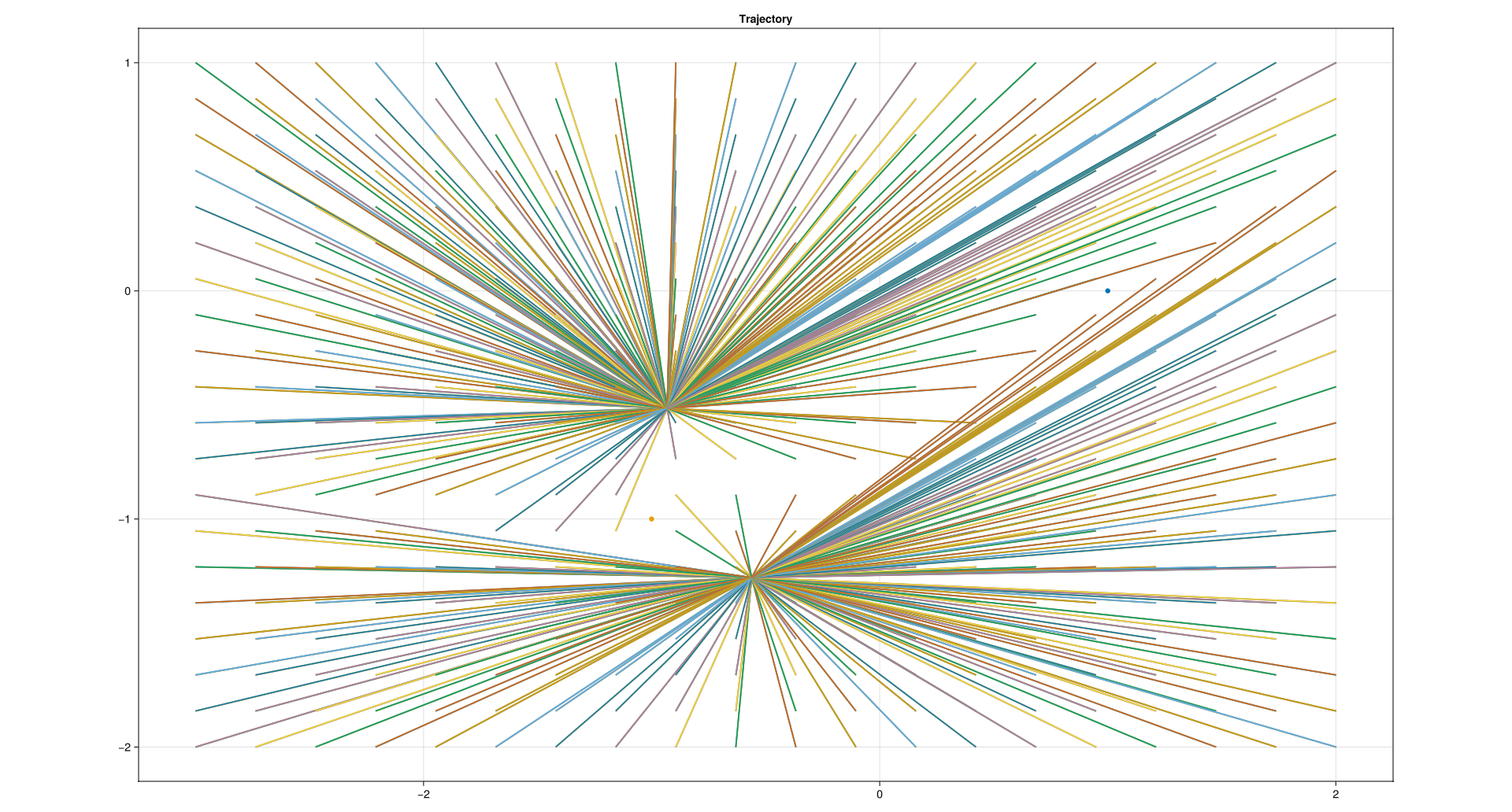
Finally, just looking at the start state and the end state:
(d) Stability of equilibrium. Given an equilibrium point, find it’s stability 2 ways: (a) With a dynamic simulation near the equilibrium; and (b) looking at the eigenvalues of the matrix describing the linearized equations of motion. Compare.
I was only able to find stable equilibriums. I was not able to use “(b) looking at the eigenvalues of the matrix describing the linearized equations of motion.”
This concludes my attempt of problem13.