problem11

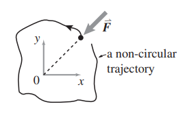
11. Central force. These two problems are both about central forces. In both cases the only force is central (directed on the particle towards the origin) and only depends on radius: \(\vec{\mathbf{F}} = −F(r)\mathbf{\hat{e}_r}\). The problems are independent, one does not follow from the other.

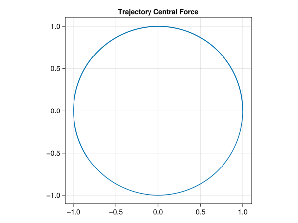
1. Find a central force law \(F(r)\) so that, comparing circular orbits of varying radii, the speed v is independent of radius.
2. By numerical experiments, and trial and error, try to find a periodic motion that is neither circular nor a straight line, for some central force besides \(F = −kr\) or \(F = \frac{−GmM}{r2}\) . a) not with a linear zero-rest length spring; b) not with inverse-square gravity; c) not circular motion; and d) not straight-line motion.
   1. In your failed searches, before you find a periodic motion, do the motions always have regular patterns or are they sometimes chaotic looking (include some pretty pictures)?
   2. Puzzle: If you use a power law, what is the minimum number loops in one complete periodic orbit (a loop is, say, a relative maximum in the radius)? How does this depend on the exponent in the power law? You probably cannot make progress with this analytically, but you can figure it out with numerical experiments

[Matlab hint: To do this properly you probably need to guess at a radial force law (most anything will work) and do numerical root finding (e.g., FSOLVE) to find initial conditions and the period of the orbit. Once you have your system you can define a function whose input is the initial conditions and the time of integration and whose output is the difference between the initial state and the final state. You can make this system ‘square’ by assuming that the particle is on the x axis in the initial state. You want to find that input which makes the output the zero vector. Pick a central force and search over initial conditions and durations. Do not use FSOLVE to search over force laws; do your orbit finding using a given force law]

../../media/problem11/problem11.png

(a) Find a central force law \(F(r)\) so that, comparing circular orbits of varying radii, the speed v is independent of radius.

Consider the relationship between centripetal force and velocity for uniform circular motion, since velocity is constant we can write:

\[F(r) = \frac{mv^2}{r}\]

\[F(r) = k\frac{m}{r}\]

Quickly drawing the trajectory for tangential initial conditions, in file ./CentralForce/src/CentralForce.jl:

u0 = [1.0;0.0;0.0;1.0]
tspan = (0.0,10.0)
m = 1.0
k = 1.0
p = Param(m, k)
ode = Physics.speedindependentofradius!
ode_prob = DifferentialEquations.ODEProblem(ode, u0, tspan, p)
sol = DifferentialEquations.solve(ode_prob)

This produces:

../../media/problem11/problem11_trajectory_central_force.png

the trajectory for non-tangential inital velocity:

TODO: add graph for velocity vs radius

(b) By numerical experiments, and trial and error, try to find a periodic motion that is neither circular nor a straight line, for some central force besides \(F = −kr\) or \(F = \frac{−GmM}{r2}\) . a) not with a linear zero-rest length spring; b) not with inverse-square gravity; c) not circular motion; and d) not straight-line motion.

First of all, I would like to note here that this was the most interesting and fun and investing problem so far in this problem set. I have spent almost 18 hours spread over 6 days on this problem.

We begin by formulating our problem:

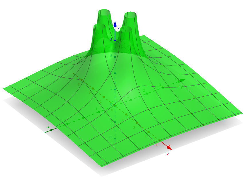
For example, an interesting central force field is this:

function dipolepowerlaw(r⃗, p)
    p₁ = [1.0, 0.0]
    p₂ = [0.0, +1.0]
    p₃ = [-1.0, 0.0]
    p₄ = [0.0, -1.0]
    points = [p₁,p₂,p₃,p₄]
    norms = norm.((r⃗ .- points))
    k = -2
    F = sum(inversepower.(norms, Ref{k}))
    return F
end
#...
function F(r⃗, p)
    dipolepowerlaw(r⃗, p)
    # speedindependentofradius(r⃗, p)
    # inversepowerlaw(r⃗, p)
    # hillinvalley(r⃗, p)
end
#...
function centralforce!(du, u, p, t)
    r⃗ = u[1:2]
    v⃗ = u[3:4]
    r̂ = normalize(r⃗)
    F⃗ = F(r⃗, p) * (-r̂)
    a⃗ = F⃗ / p.m
    du[1:2] = v⃗
    du[3:4] = a⃗
end

The graph for this magnitude of this central force field looks like this:

Dipole power law

For any such function centralforce!(du, u::State, p::Parameters, tend:Time)::State, we want to find a \(\vec{u}_0\) such that, for \(\vec{u}_t\) = DifferentialEquations.solve(odeprob)[end]

\[\vec{u}_t - \vec{u}_0 = \vec{0}\]

Which is equivalent to finding a zero to the following function f, in file ./CentralForce/src/RootFinding.jl:

f(z⃗₀, p) = begin
    tol = 1e-12
    u⃗₀ = z⃗₀[1:end-1]
    tend = z⃗₀[end]
    dynamics_prob = ProblemSetup.create_problem(ProblemSetup.ode!, u⃗₀, tend, p)
    dynamics_sol = DifferentialEquations.solve(dynamics_prob; abstol=tol, reltol=tol, save_everystep=false)
    u⃗ₜ = dynamics_sol.u[end]
    Δu⃗ = u⃗ₜ - u⃗₀
    phasecondition = u⃗₀[2] # crosses the x axis
    # v⃗₀ = u⃗₀[3:4]
    # limit = 0.1
    # if LinearAlgebra.norm(v⃗₀) < limit || tend < 0.1
    #     return zeros(5) .+ 1.0
    # end
    # Δu⃗
    return [Δu⃗; phasecondition]
end

One challenge I overcame after much thinking is regarding the phasecondition, the number of variables to solve for should equal the number of equations, earlier the input dimension was five: \((x, y, vx, vy, tend)\) while the output dimension was four (Δx, Δy, Δvx, Δvy).

The following is the question I asked in a julia help group online:

In the non-linear root finding, does the input dimension have to match the output dimensions?

Right now I have input output dimension as 5, 4 respectively. input (5): (x, y, vx, vy, tend) output (4): (Δx, Δy, Δvx, Δvy )

Somehow I feel this is not ideal. The system of nonlinear equations feels under defined. So, to correct this I added the constraint of solution roots should start on the y axis, i.e x = 0

In my system this is equivalent to:

f(z⃗₀, p) = begin
    tol = 1e-12

    u⃗₀ = z⃗₀[1:end-1]
    tend = z⃗₀[end]

    dynamics_prob = ProblemSetup.create_problem(ProblemSetup.ode!, u⃗₀, tend, p)
    dynamics_sol = DifferentialEquations.solve(dynamics_prob; abstol=tol, reltol=tol, save_everystep=false)
    u⃗ₜ = dynamics_sol.u[end]
    Δu⃗ = u⃗ₜ - u⃗₀

    phasecondition = u⃗₀[2] # crosses the x axis

    # v⃗₀ = u⃗₀[3:4]
    # limit = 0.1
    # if LinearAlgebra.norm(v⃗₀) < limit || tend < 0.1
    #     return zeros(5) .+ 1.0
    # end
    # return Δu⃗
    return [Δu⃗; phasecondition]
end

But now the root finder is giving me this warning and gets stuck:

 Warning: Interrupted. Larger maxiters is needed. If you are using an integrator for non-stiff ODEs or an automatic switching algorithm (the default), you may want to consider using a method for stiff equations. See the solver pages for more details (e.g. https://docs.sciml.ai/DiffEqDocs/stable/solvers/ode_solve/#Stiff-Problems).
└ @ SciMLBase ~/.julia/packages/SciMLBase/cwnDi/src/integrator_interface.jl:589
┌ Warning: Potential Rank Deficient Matrix Detected. Attempting to solve using Pivoted QR Factorization.
└ @ NonlinearSolveBaseLinearSolveExt ~/.julia/packages/NonlinearSolveBase/yZeYz/ext/NonlinearSolveBaseLinearSolveExt.jl:33
┌ Warning: At t=1.619487808996462e18, dt was forced below floating point epsilon 256.0, and step error estimate = 1.7742389634428446. Aborting. There is either an error in your model specification or the true solution is unstable (or the true solution can not be represented in the precision of Float64).
└ @ SciMLBase ~/.julia/packages/SciMLBase/cwnDi/src/integrator_interface.jl:623
┌ Warning: Interrupted. Larger maxiters is needed. If you are using an integrator for non-stiff ODEs or an automatic switching algorithm (the default), you may want to consider using a method for stiff equations. See the solver pages for more details (e.g. https://docs.sciml.ai/DiffEqDocs/stable/solvers/ode_solve/#Stiff-Problems).
└ @ SciMLBase ~/.julia/packages/SciMLBase/cwnDi/src/integrator_interface.jl:589
┌ Warning: Potential Rank Deficient Matrix Detected. Attempting to solve using Pivoted QR Factorization.
└ @ NonlinearSolveBaseLinearSolveExt ~/.julia/packages/NonlinearSolveBase/yZeYz/ext/NonlinearSolveBaseLinearSolveExt.jl:33
┌ Warning: At t=1.619487808996462e18, dt was forced below floating point epsilon 256.0, and step error estimate = 1.7742389634428446. Aborting. There is either an error in your model specification or the true solution is unstable (or the true solution can not be represented in the precision of Float64).
└ @ SciMLBase ~/.julia/packages/SciMLBase/cwnDi/src/integrator_interface.jl:623
Is this because the phasecondition is linearly dependent to the state vector, I don't feel that is the case. What is going on?

The answer I got was by @romanveltz: “BifurcationKit does all that already”.

TODO: Explore how BifurcationKit.jl achieves non-linear root finding.

We can formulate the solution to this either in an optimization way, or a root finding way.

One way to feed the initial conditions to the root solver is to keep doubling the norm of the initial condition vector, this is to avoid trivial roots: \(tend = 0\) or \(v_0 = 0\)

In julia, I use the NonlinearSolver. In file ./CentralForce/src/RootFinding.jl:

function strategy_exponentiate()
    randunitvec() = begin
        θ = 2π*rand()
        r = √(rand())
        r*[cos(θ); sin(θ)]
    end
    
    
    tend_limit = 16000
    v₀_limit = 1600
    tend_init = 1.0
    v₀_init = 1.0
    factor = 2
    periodic_sol = Vector{Float64}(undef, 5)
    istrivial_tend_init = true
    istrivial_v₀_init = true
    varsinlimit() = begin
        ((tend_init < tend_limit) && (v₀_init < v₀_limit))
    end
    varstrivial() = begin
        (istrivial_tend_init || istrivial_v₀_init)
    end
    while varsinlimit() && varstrivial()
        # local tend_init, istrivial_tend_init, v₀_init, istrivial_v₀_init, periodic_sol
    
        u⃗₀_init = [100*randunitvec(); v₀_init * randunitvec()]
        z⃗₀_init = [u⃗₀_init; tend_init]
    
        root_prob = NonlinearSolve.NonlinearProblem(RootFinding.f, z⃗₀_init, ProblemSetup.p)
        root_sol = NonlinearSolve.solve(root_prob)
        println("Solver status: ", root_sol.retcode)
        println("Residual norm: ", LinearAlgebra.norm(root_sol.resid))
        u⃗₀_sol = root_sol[1:end - 1]
        tend_sol = root_sol[end]
        v⃗₀_sol = u⃗₀_sol[3:4]
        v₀_sol = LinearAlgebra.norm(v⃗₀_sol)
        println(" ; root:tend_sol ", tend_sol, " ; root:v₀_sol ", v₀_sol)
        lowerlimit = 0.1
        istrivial_tend_init = (tend_sol < lowerlimit)
        istrivial_v₀_init = (v₀_sol < lowerlimit)
        if varstrivial()
            tend_init *= factor
            v₀_init *= factor
        else
            println("Congratulations, found non-trivial periodic orbit")
            periodic_sol = root_sol
        end
        println("something trivial? : ", varstrivial())
    end
    
    # periodic_sol = 
    # u⃗₀_periodic = periodic_sol[1:4]
    # tend_periodic = periodic_sol[5]
    # # plot the periodic solution
    # plot_solution(ode!, u⃗₀_periodic, tend_periodic, p)
    return periodic_sol
end

Another strategy is to sample and pass every point in a mesh as a initial state to the solver, in the same file

function strategy_meshcheck()
    K = 100.0
    N = 10
    meshrange = range(-K, K, N)
    meshtime = range(0.0, K, N)
    count = 0
    roots = []
    println("Hello")
    for x in meshrange
        for y in meshrange
            for vx in meshrange
                for vy in meshrange
                    for t in meshtime
                        global count
                        r = LinearAlgebra.norm([x;y])
                        v = LinearAlgebra.norm([vx;vy])
                        if r < 1.0 || v < 1.0 || t < 1.0
                            println("skipping small cases")
                            continue
                        end
                        z⃗₀_init = [x; y; vx; vy; t]

                        root_prob = NonlinearSolve.NonlinearProblem(RootFinding.f, z⃗₀_init, ProblemSetup.p)
                        println(z⃗₀_init)
                        root_sol = NonlinearSolve.solve(root_prob)

                        count += 1
                        percentage = 100*count / (N^length(z⃗₀_init))
                        println(percentage, "% completed")

                        if root_sol.retcode == NonlinearSolve.ReturnCode.Success
                            push!(roots, root_sol)
                        end
                    end
                end
            end
        end
    end
    println("Successfuly converged solutions: ", roots)
end

The root finder was not converging for me for these.

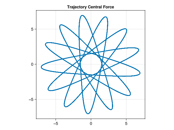
But still with a bit of intuition I was able to find a non trivial Central Force Field with a non trivial periodic orbit, ./CentralForce/src/Physics.jl:

For the following force field:

#...
function hillinvalley(r⃗, p)
    r = norm(r⃗)
    σ = 5
    a = 5
    e = a*exp(-σ*r^2)
    p = r^2
    F = e+p #-a
end
#...

The graph of the magnitude of this force field:

problem11-hillinvalley-graph.png

With the follwoing intiial conditions, in file ./CentralForce/src/CentralForce.jl:

#...
tol = 1e-12
function plot_solution(u⃗₀, tend)
    ode_prob = ProblemSetup.create_problem(ProblemSetup.ode!, u⃗₀, tend, ProblemSetup.p)
    sol = DifferentialEquations.solve(ode_prob, DifferentialEquations.Tsit5(); abstol=tol, reltol=tol, saveat=0.01)
    trajectory = Visualization.plot_trajectory(sol)
    GLMakie.save("./trajectory-solution.png", trajectory)
    GLMakie.display(trajectory)
end
#...
tend = 50000.0
r⃗ = [5, 5]
v = 5.4225
v⃗ = [-v, v]
u⃗₀ = [r⃗; v⃗]
plot_solution(u⃗₀, tend)

We get the surely periodic orbit, ‘surely periodic’ meaning I dont have an analytical proof yet but have tested it for tend=5000:

problem11-hillinvalley-trajectory.png

The inconsistent use of code blocks and \(math blocks\) was an intentional fast.